Sometimes people ask me how the examples of my plotting functions I show here can be reproduced without having a SPSS data set (or at least, without having the data set I use because it’s not public yet). So I started to write some examples that run “out of the box” and which I want to present you here. Furthermore, two new plotting functions are introduced: plotting correlations and plotting proportional tables on a percentage scale.

As always, you can find the latest version of my R scripts on my download page.

Following plotting functions will be described in this posting:

• Plotting proportional tables: sjPlotPropTable.R
• Plotting correlations: sjPlotCorr.R
• Plotting frequencies: sjPlotFrequencies.R
• Plotting grouped frequencies: sjPlotGroupFrequencies.R
• Plotting linear model: sjPlotLinreg.R
• Plotting generalized linear models: sjPlotOdds.R

Please note that I have changed function and parameter names in order to have consistent, logical names across all functions!

At the end of this posting you will find some explanation on the different parameters that allow you to fit the plotting results to your needs…

Please note that additional packages besides ggplot2 maybe have to be installed!
You may need following packages, depending on which script you run:

• plyr
• quantreg
• scales
• reshape2
• vcd

Plotting proportional tables: sjPlotPropTable.R
The idea for this function came up when I saw the distribution of categories (or factor levels) within one group or variable, that sum up to 100% – typically shown as stacked bars. So I wrote a script that shows the cross tabulation of two variables and either show column or row percentage calculations.

First, load the script and create two random variables:

source("sjPlotPropTable.R")
grp <- sample(1:4, 100, replace=T)
y <- sample(1:3, 100, replace=T)

The simplest way to produce a plot is following (note that, due to random sampling, your plots my look different!):

sjp.xtab(y, grp)

Proportional table of two variables, column percentages, with “Total” column.

You can specify axis and legend labels:

sjp.xtab(y, grp,
         axisLabels.x=c("low", "mid", "high"),
         legendLabels=c("Grp 1", "Grp 2", "Grp 3", "Grp 4"))

Proportional table, column percentages, with assigned labels.

If you want row percentages, you can use stacked bars because each group sums up to 100%:

sjp.xtab(y, grp,
         tableIndex="row",
         barPosition="stack",
         flipCoordinates=TRUE)

Proportional table, stacked bars of row percentages,

Plotting correlations: sjPlotCorr.R
A very quick way of plotting a correlation heat map can be found in this blog. I had a similar idea in mind for some time and decided to write a small function that allows some tweaking of the produced plot like different colors indicating positive or negative correlations and so on.

Again, at first load the script and create a random sample:

source("sjPlotCorr.R")
df <- as.data.frame(cbind(rnorm(10),
                    rnorm(10),
                    rnorm(10),
                    rnorm(10),
                    rnorm(10)))

You can either pass a data frame as parameter or a computed correlation object as well. If you use a data frame, following correlation will be computed:

cor(df, method="spearman"
    use="pairwise.complete.obs")

The simple function call is:

sjp.corr(df)

Correlation matrix of all variables in a data frame.

This gives you a correlation map with both circle size and color intensity indicating the strength of the correlations. You can also plot tiles, which looks more like a heat map, if you prefer:

sjp.corr(df, type="tile", theme="none")

Tiled correlation matrix without background theme.

Plotting frequencies: sjPlotFrequencies.R
There is already a posting which demonstrates this script, however, since it uses a SPSS data set, I want to give short examples that run out of the box here.

Load the script:

source("sjPlotFrequencies.R")

A simple bar chart:

sjp.frq(ChickWeight$Diet)

Simple bar chart of frequencies.

A box plot:

sjp.frq(ChickWeight$weight, type="box")

A simple box plot with median and mean dot.

A violin plot:

sjp.frq(ChickWeight$weight, type="v")

A violin plot (density curve estimation) with box plot inside.

And finally, a histrogram with mean and standard deviation:

sjp.frq(discoveries, type="hist", showMeanIntercept=TRUE)

Histogram with mean intercept and standard deviation range.

Plotting grouped frequencies: sjPlotGroupFrequencies.R
The grouped frequencies script has also been described in a separate posting.

Load the script:

source("sjPlotGroupFrequencies.R")

Grouped bars using the ChickenWeight data set. Note that due to random sampling, your figure may look different:

sjp.grpfrq(sample(1:3, length(ChickWeight$Diet), replace=T),
           as.numeric(ChickWeight$Diet),
           barSpace=0.2)

Grouped bars.

Grouped box plots. Note that this plot automatically computes the Mann-Whitney-U-test for the relation of each two subgroups. The tested groups are indicated by the subscriped numbers after the “p”:

sjp.grpfrq(ChickWeight$weight,
           as.numeric(ChickWeight$Diet),
           type="box")

Grouped box plots, showing the Weight distribution, divided into 4 random groups.

Grouped histogram:

sjp.grpfrq(discoveries,
           sample(1:3, length(discoveries), replace=T),
           type="hist",
           showValueLabels=FALSE,
           showMeanIntercept=TRUE)

Grouped histogram of “Discoveries”, divided into three random subgroups, including mean intercepts for each group.

Plotting linear model: sjPlotLinreg.R
Plotting (generalized) linear models have also already been described in a posting, so I will keep it short here and just give a running example:

source("sjPlotLinreg.R")
fit <- lm(airquality$Ozone ~ airquality$Wind +
          airquality$Temp +
          airquality$Solar.R)
sjp.lm(fit, gridBreaksAt=2)

Beta coefficients (blue) and standardized beta coefficients (red) from a linear model.

Plotting generalized linear models: sjPlotOdds.R

source("sjPlotOdds.R")
y <- ifelse(swiss$Fertility<median(swiss$Fertility), 0, 1)
fitOR <- glm(y ~ swiss$Examination + 
             swiss$Education + 
             swiss$Catholic + 
             swiss$Infant.Mortality, 
             family=binomial(link="logit"))
sjp.glm(fitOR, transformTicks=TRUE)

Odds ratios.

Which parameters can be changed?
There is, depending on the function, a long list of parameters that can be changed to tweak the figure you want to produce. If you use editors like RStudio, you can press ctrl+space inside a function call to access a list of all available parameters of a function. All available parameters are documented at the beginning of each script (and if not, please let me know so I can complete the documentation).

Three examples of what you can modify in your plot:

Labels
Axis labels can be changed with the axisLabel.x or axisLabel.y parameter, depending on where labels appear (for instance, if you have frequencies, you use the .x, if you plot linear models, you use .y to change the labels). The size and color of labels can be changed with axisLabelSize and axisLabelColor. Value labels (labels inside the diagram), however, are manipulated with valueLabels, valueLabelSize and valueLabelColor. The same pattern applies to legend labels.

Showing / hiding elements
Many labels, values or graphical elements can be shown or hidden. showAxisLabels.x shows/hides the variable labels on the x-axis. showValueLabels shows/hides the value labels inside a diagram etc.

Diagram type
With the type parameter you can specifiy the type of diagram. E.g. the sjPlotFrequencies offers histograms, bars, box plots etc. Just specifiy the desired type with this parameter.

Last remarks
In case you want to apply the above shown functions on your (imported) data sets, you also may find this posting helpful.

This script was almost written on parallel to the sjPlotCorr script because it uses a very similar ggplot-base. However, there’s also a very nice posting over at Martin’s Bio Blog which show alternative approaches on plotting PCAs.

Anyway, if you download the sjPlotPCA.R script, you can easily plot a PCA with varimax rotation like this:

likert_4 <- data.frame(sample(1:4, 500, replace=T, prob=c(0.2,0.3,0.1,0.4)),
                       sample(1:4, 500, replace=T, prob=c(0.5,0.25,0.15,0.1)),
                       sample(1:4, 500, replace=T, prob=c(0.4,0.15,0.25,0.2)),
                       sample(1:4, 500, replace=T, prob=c(0.25,0.1,0.4,0.25)),
                       sample(1:4, 500, replace=T, prob=c(0.1,0.4,0.4,0.1)),
                       sample(1:4, 500, replace=T,),
                       sample(1:4, 500, replace=T, prob=c(0.35,0.25,0.15,0.25)))
colnames(likert_4) <- c("V1", "V2", "V3", "V4", "V5", "V6", "V7")
source("../lib/sjPlotPCA.R")
sjp.pca(likert_4)

So, all you have to do is creating a data frame where each column represents one variable / case and pass this data frame to the function. This will result in something like this:

PCA of 7 variables resulting in 3 extracted factors (varimax rotation). Cronbach’s Alpha value of each “factor scale” printed at bottom.

The script automatically calculates the Cronbach’s Alpha value for each “factor scale”, assuming that the variables with the highest factor loading belongs to this factor. The amount of factors is calculated according to the Kaiser criterion. You can also create a plot of this calcuation by setting the parameter plotEigenvalues=TRUE.

The next small example shows two plots and uses a computed PCA as paramater:

pca <- prcomp(na.omit(likert_4), retx=TRUE, center=TRUE, scale.=TRUE)
sjp.pca(pca, plotEigenvalues=TRUE, type="circle")

Eigenvalue plot determining amount of factors (Kaiser criterion)

Same PCA plot as above, with PCA object instead of data frame as parameter.

That’s it! The source is available on my download page.

Update Thanks to Forrest for finding and fixing a bug. Scripts have been updated!

Update 2 Scripts have been updated because item ordering was still buggy. Hope everything is fixed now. Very helpful in this context was the new debug feature of RStudio, that also keeps track of all variables and their content and allows step-by-step execution of your code.

First of all, credits for this script must go to Ethan Brown, whose ideas for creating Likert scales like plots with ggplot built the core of my sjPlotLikert.R-script.

All I did was some visual tweaking like having positive percentage values on both sides of the x-axis, adding value labels and so on… You can pass a lot of different parameters to modify the graphical output. Please refer to my blog postings on R to get some impressions of how to tweak the plot (and/or look into the script header, which includes a description of all parameters).

Now to some examples:

likert_2 <- data.frame(as.factor(sample(1:2, 500, replace=T, prob=c(0.3,0.7))),
                       as.factor(sample(1:2, 500, replace=T, prob=c(0.6,0.4))),
                       as.factor(sample(1:2, 500, replace=T, prob=c(0.25,0.75))),
                       as.factor(sample(1:2, 500, replace=T, prob=c(0.9,0.1))),
                       as.factor(sample(1:2, 500, replace=T, prob=c(0.35,0.65))))
levels_2 <- list(c("Disagree", "Agree"))
items <- list(c("Q1", "Q2", "Q3", "Q4", "Q5"))
source("sjPlotLikert.R")
sjp.likert(likert_2, legendLabels=levels_2, axisLabels.x=items, orderBy="neg")

2-items Likert scale, ordered by “negative” categories.

likert_4 <- data.frame(as.factor(sample(1:4, 500, replace=T, prob=c(0.2,0.3,0.1,0.4))),
                       as.factor(sample(1:4, 500, replace=T, prob=c(0.5,0.25,0.15,0.1))),
                       as.factor(sample(1:4, 500, replace=T, prob=c(0.25,0.1,0.4,0.25))),
                       as.factor(sample(1:4, 500, replace=T, prob=c(0.1,0.4,0.4,0.1))),
                       as.factor(sample(1:4, 500, replace=T, prob=c(0.35,0.25,0.15,0.25))))
levels_4 <- list(c("Strongly disagree", "Disagree", "Agree", "Strongly Agree"))
items <- list(c("Q1", "Q2", "Q3", "Q4", "Q5"))
source("sjPlotLikert.R")
sjp.likert(likert_4, legendLabels=levels_4, axisLabels.x=items)

4-category-Likert-scale, ordered by items.

likert_6 <- data.frame(as.factor(sample(1:6, 500, replace=T, prob=c(0.2,0.1,0.1,0.3,0.2,0.1))),
                       as.factor(sample(1:6, 500, replace=T, prob=c(0.15,0.15,0.3,0.1,0.1,0.2))),
                       as.factor(sample(1:6, 500, replace=T, prob=c(0.2,0.25,0.05,0.2,0.2,0.2))),
                       as.factor(sample(1:6, 500, replace=T, prob=c(0.2,0.1,0.1,0.4,0.1,0.1))),
                       as.factor(sample(1:6, 500, replace=T, prob=c(0.1,0.4,0.1,0.3,0.05,0.15))))
levels_6 <- list(c("Very strongly disagree", "Strongly disagree", "Disagree", "Agree", "Strongly Agree", "Very strongly agree"))
items <- list(c("Q1", "Q2", "Q3", "Q4", "Q5"))
source("sjPlotLikert.R")
sjp.likert(likert_6, legendLabels=levels_6, barColor="brown", axisLabels.x=items, orderBy="pos")

6-category-Likert-scale with different color set and ordered by “positive” categories.

If you need to plot stacked frequencies that have no “negative” and “positive”, but only one direction, you can also use my sjPlotStackFrequencies.R script. Given that you use the likert-data frames from the above examples, you can run following code to plot stacked frequencies for scales that range from “low” to “high” and not from “negative” to “positive”.

levels_42 <- list(c("Independent", "Slightly dependent", "Dependent", "Severely dependent"))
levels_62 <- list(c("Independent", "Slightly dependent", "Dependent", "Very dependent", "Severely dependent", "Very severely dependent"))
source("lib/sjPlotStackFrequencies.R")
sjp.stackfrq(likert_4, legendLabels=levels_42, axisLabels.x=items)
sjp.stackfrq(likert_6, legendLabels=levels_62, axisLabels.x=items)

This produces following two plots:

Stacked frequencies of 4-category-items.

Stacked frequencies of 6-category-items.

That’s it!

I haven’t used interaction terms in (generalized) linear model quite often yet. However, recently I have had some situations where I tried to compute regression models with interaction terms and was wondering how to interprete the results. Just looking at the estimates won’t help much in such cases.

One approach used by some people is to compute the regressions with subgroups for each category of one interaction term. Let’s say predictor A has a 0/1 coding and predictor B is a continuous scale from 1 to 10, you fit a model for all cases with A=0 (hence excluding A from the model, no interaction of A and B), and for all cases with A=1 and compare the estimates of predictor B in each fitted model. This may give you an impression under which condition (i.e. in which subgroup) A has a stronger effect on B (higher interaction), but of course you don’t have the correct estimate values compared to a fitted model that includes both the interaction terms A and B.

Another approach is to calculate the results of y by hand, using the formula:
y = b0 + b1*predictorA + b2*predictorB + b3*predictorA*predictorB
This is quite complex and time-comsuming, especially if both predictors have several categories. However, this approach gives you a correct impression of the interaction between A and B. I investigated further on this topic and found this nice blogpost on interpreting interactions in regression (and a follow up), which explains very well how to calculate and interprete interaction terms.

Based on this knowledge, I thought of an automatization of calculating and visualizing interaction terms in linear models using R and ggplot.

Downloading the script

You can download the script sjPlotInteractions.R from my script page. The function sjp.lmint requires at least one parameter: a fitted linear model object, including interaction terms.

What this script does:

1. it extracts all significant interactions
2. from each of these interactions, both terms (or predictors) are analysed. The predictor with the higher number of unique values is chosen to be printed on the x-axis.
3. the predictor with fewer numbers of unique values is printed along the y-axis.
4. Two regression lines are calulated:
   1. every y-value for each x-value of the predictor on the x-axis is calculated according to the formula y = b0 + b(predictorOnXAxis)*predictorOnXAxis + b3*predictorOnXAxis*predictorOnYAxis, using the lowest value of predictorOnYAxis
   2. every y-value for each x-value of the predictor on the x-axis is calculated according to the formula y = b0 + b(predictorOnXAxis)*predictorOnXAxis + b3*predictorOnXAxis*predictorOnYAxis, using the highest value of predictorOnYAxis
5. the above steps are repeated for each significant interactions.

Now you should have a plot for each interaction that shows the minimum impact (or in case of 0/1 coding, the absence) of predictorYAxis on predictorXAxis according to y (the response, or dependent variable) as well as the maximum effect (or in case of 0/1 coding, the presence of predictorYAxis).

Some examples…

source("sjPlotInteractions.R")
fit <- lm(weight ~ Time * Diet, data=ChickWeight, x=T)
summary(fit)

This is the summary of the fitted model. We have three significant interactions.

Call:
lm(formula = weight ~ Time * Diet, data = ChickWeight, x = T)

Residuals:
     Min       1Q   Median       3Q      Max 
-135.425  -13.757   -1.311   11.069  130.391 

Coefficients:
            Estimate Std. Error t value Pr(>|t|)    
(Intercept)  30.9310     4.2468   7.283 1.09e-12 ***
Time          6.8418     0.3408  20.076  < 2e-16 ***
Diet2        -2.2974     7.2672  -0.316  0.75202    
Diet3       -12.6807     7.2672  -1.745  0.08154 .  
Diet4        -0.1389     7.2865  -0.019  0.98480    
Time:Diet2    1.7673     0.5717   3.092  0.00209 ** 
Time:Diet3    4.5811     0.5717   8.014 6.33e-15 ***
Time:Diet4    2.8726     0.5781   4.969 8.92e-07 ***
---
Signif. codes:  0 ‘***’ 0.001 ‘**’ 0.01 ‘*’ 0.05 ‘.’ 0.1 ‘ ’ 1

Residual standard error: 34.07 on 570 degrees of freedom
Multiple R-squared:  0.773,	Adjusted R-squared:  0.7702 
F-statistic: 277.3 on 7 and 570 DF,  p-value: < 2.2e-16

As example, only one of these three plots is shown.

sjp.lmint(fit)

Interaction of Time and Diet

If you like, you can also plot value labels.

sjp.lmint(fit, showValueLabels=T)

Interaction of Time and Diet, with value labels

In case you have at least one dummy variable (0/1-coded) as predictor, you should get a clear linear line. However, in case of two scales, you might have “curves”, like in the following example:

source("lib/sjPlotInteractions.R")
fit <- lm(Fertility ~ .*., data=swiss, na.action=na.omit, x=T)
summary(fit)

The resulting fitted model:

Call:
lm(formula = Fertility ~ . * ., data = swiss, na.action = na.omit, 
    x = T)

Residuals:
    Min      1Q  Median      3Q     Max 
-8.7639 -3.8868 -0.6802  3.1378 14.1008 

Coefficients:
                               Estimate Std. Error t value Pr(>|t|)    
(Intercept)                  253.976152  67.997212   3.735 0.000758 ***
Agriculture                   -2.108672   0.701629  -3.005 0.005217 ** 
Examination                   -5.580744   2.750103  -2.029 0.051090 .  
Education                     -3.470890   2.683773  -1.293 0.205466    
Catholic                      -0.176930   0.406530  -0.435 0.666418    
Infant.Mortality              -5.957482   3.089631  -1.928 0.063031 .  
Agriculture:Examination        0.021373   0.013775   1.552 0.130915    
Agriculture:Education          0.019060   0.015229   1.252 0.220094    
Agriculture:Catholic           0.002626   0.002850   0.922 0.363870    
Agriculture:Infant.Mortality   0.063698   0.029808   2.137 0.040602 *  
Examination:Education          0.075174   0.036345   2.068 0.047035 *  
Examination:Catholic          -0.001533   0.010785  -0.142 0.887908    
Examination:Infant.Mortality   0.171015   0.129065   1.325 0.194846    
Education:Catholic            -0.007132   0.010176  -0.701 0.488650    
Education:Infant.Mortality     0.033586   0.124199   0.270 0.788632    
Catholic:Infant.Mortality      0.009919   0.016170   0.613 0.544086    
---
Signif. codes:  0 ‘***’ 0.001 ‘**’ 0.01 ‘*’ 0.05 ‘.’ 0.1 ‘ ’ 1

Residual standard error: 6.474 on 31 degrees of freedom
Multiple R-squared:  0.819,	Adjusted R-squared:  0.7314 
F-statistic: 9.352 on 15 and 31 DF,  p-value: 1.077e-07

And the plot:

sjp.lmint(fit)

If you prefer, you can smoothen the line by using smooth="loess" parameter:

sjp.lmint(fit, smooth="loess")

loess-smoothed interaction plot

Or you can force to print a linear line by using smooth="lm" parameter:

sjp.lmint(fit, smooth="lm")

Plot with forced linear smoothing

I’m not sure whether I used the right terms in titles and legends (“effect on… under min and max interaction…”). If you have suggestions for alternative descriptions of title and legends that are “statistically” more correct, please let me know!

That’s it!

This weekend I had some time to deal with package building in R. After some struggling, I now managed to setup RStudio, Roxygen and MikTex properly so I can compile my collection of R-scripts into a package that even succeeds the package check.

Downloads (package and manual) as well as package description are available at the package information page!

Since the packages successfully passed the package check and a manual could also be created, I’ll probably submit my package to the CRAN. Currently, I’m only able to compile the source and the Windows binaries of the package, because at home I use RStudio on my Mac with OS X 10.9 Mavericks. It seems that there’s an issue with the GNU Tar on Mavericks, which is needed to compile the OS X binaries… I’m not sure whether it’s enough to just submit the source the the CRAN.

Anyway, please check out my package and let me know if you encounter any problems or if you have suggestions on improving the documentation etc.

Open questions

• How do I write an “ü” in the R-documentation (needed for my family name in author information)? The documentation is inside the R-files, the RD-files are created using Roxygen.
• How do I include datasets inside an R-package? I would like to include an SPSS-dataset (.sav-File), so I can make the examples of my sji.XYZ functions running… (currently they’re outcommented so the package will compile and pass its check properly)
• How to include a change log inside R-packages?

I’d like to announce the release of version 0.7 of my R package for data visualization and give a small overview of this package (download and installation instructions can be found on the package page).

What does this package do?
In short, the functions in this package mostly do two things:

1. compute basic or advanced statistical analyses
2. plot the results as ggplot-diagram

However, meanwhile the amount of functions has increased, hence you’ll also find some utility functions beside the plotting functions.

How does this package help me?
Basically, this package either helps those users…

• who have difficulties using and/or understanding all possibilities that ggplot offers to create plots, simply by providing intuitive function parameters, which allow for manipulating the appearance of plots; or
• who don’t want to set up complex ggplot-object each time from the scratch.

Furthermore, for advanced ggplot-users, the functions can return the prepared ggplot-object, which than can be manipulated even further (for instance, if you wish to specify certain parameters that cannot be modified via the sjPlot package).

What are all these functions about?
There’s a certain naming convention for the functions:

• sjc – collection of functions useful for carrying out cluster analyses
• sji – collection of functions for data import and manipulation
• sjp – collection plotting functions, the “core” of this package
• sjt – collection of function that create (HTML) table outputs (instead of ggplot-graphics
• sju – collection of statistical utility functions

Use cases?

• You can plot results of Anova, correlations, histograms, box plots, bar plots, (generalized) linear models, likert scales, PCA, proportional tables as bar chart etc.
• You can create plots to analyse model assumptions (lm, glm), predictor interactions, multiple contigency tables etc.
• With the import and utility functions, you can, for instance, extract beta coefficients of linear models, convert numeric scales into grouped factors, perform statistical tests, import SPSS data sets (and retrieve variable and value labels from the importet data), convert factors to numeric variables (and vice versa)…

Final remarks
At the bottom of my package page you’ll find some examples of selected functions that have been published on this blog before I created the package. Furthermore, the package includes a sample dataset from one of my research projects. Once the package is installed, you can test each function by running the examples. All news and recent changes can be found in the NEWS section of the package help (type ?sjPlot to access the help file inside R).

I tried to write a very comprehensive documentation for each function and their parameters, hopefully this will help you using my package…

Any comments, suggestions etc. are very welcome!

Since version 0.8, my package for data visualization using ggplot has been released on the Comprehensive R Archive Network (CRAN), which means you can simply install the package with install.packages("sjPlot").

Last week, version 0.9 was released. Binaries are already available for OS X and Windows, and source code for Linux. Further updates will no longer be announced on this blog (except for new functions which may be described in dedicated blog postings), so please use the update function in order make sure you are using the latest package version.

It’s been a while since a user of my plotting-functions asked whether it would be possible to compare multiple (generalized) linear models in one graph (see comment). While it is already possible to compare multiple models as table output, I now managed to build a function that plots several (g)lm-objects in a single ggplot-graph.

The following examples are based on a development snapshot of my sjPlot package. You can download the script of the sjp.glmm function here (the latest release of my package probably has to be installed to run the script due to dependencies on other help-functions that are not included in the script). Please note that this script will not be updated! It will be included in the next update of my package!

Once you’ve compiled the script, you can run one of the examples provided in the function’s documentation:

# prepare dummy variables for binary logistic regression
y1 <- ifelse(swiss$Fertility<median(swiss$Fertility), 0, 1)
y2 <- ifelse(swiss$Infant.Mortality<median(swiss$Infant.Mortality), 0, 1)
y3 <- ifelse(swiss$Agriculture<median(swiss$Agriculture), 0, 1)

# Now fit the models. Note that all models share the same predictors
# and only differ in their dependent variable (y1, y2 and y3)
fitOR1 <- glm(y1 ~ swiss$Education+swiss$Examination+swiss$Catholic,
              family=binomial(link="logit"))
fitOR2 <- glm(y2 ~ swiss$Education+swiss$Examination+swiss$Catholic,
              family=binomial(link="logit"))
fitOR3 <- glm(y3 ~ swiss$Education+swiss$Examination+swiss$Catholic,
              family=binomial(link="logit"))

# plot multiple models
sjp.glmm(fitOR1, fitOR2, fitOR3)

Thanks to the help of a stackoverflow user, I now know that the order of aes-parameters matters in case you have dodged positioning of geoms on a discrete scale. An example: I use following code in my function ggplot(finalodds, aes(y=OR, x=xpos, colour=grp, alpha=pa)) to apply different colours to each model and setting an alpha-level for geoms depending on the p-level. If the alpha-aes would appear before the colour-aes, the order of lines representing a model may be different for different x-values (see stackoverflow example).

Another more appealing example (not reproducable, since it relies on data from a current research project):

And finally an example where p-levels are represented by different shapes and non-significant odds have a lower alpha-level:

This function and an equivalent for linear models will be included in the next update of my sjPlot package.

Inspired by these two postings, I thought about including a function in my package for simply creating scatter plots.

In my package, there’s a function called sjp.scatter for creating scatter plots. To reproduce these examples, first load the package and then attach the sample data set:

data(efc)

The simplest function call is by just providing two variables, one for the x- and one for the y-axis:

sjp.scatter(efc$c160age, efc$e17age)

which plots following graph:

If you have continuous variables with a larger scale, you shouldn’t have problems with overplotting or overlaying dots. However, this problem usually occurs, if you have variables with just a few categories (factor levels). The function automatically estimates the amount of overlaying dots and then automatically jitters them, like in following example, which also includes a marginal rug-plot:

sjp.scatter(efc$e16sex,efc$neg_c_7, efc$c172code, showRug=TRUE)

The same plot, when auto-jittering is turned off, would look like this:

sjp.scatter(efc$e16sex,efc$neg_c_7, efc$c172code,
            showRug=TRUE, autojitter=FALSE)

You can also add a grouping variable. The scatter plot is then “divided” into as many groups as indicated by the grouping variable. In the next example, two variables (elder’s and carer’s age) are grouped by different dependency levels of the elderly. Additionally, a fitted line for each group is plotted:

sjp.scatter(efc$c160age,efc$e17age, efc$e42dep, title="Scatter Plot",
            legendTitle=sji.getVariableLabels(efc)['e42dep'],
            legendLabels=sji.getValueLabels(efc)[['e42dep']],
            axisTitle.x=sji.getVariableLabels(efc)['c160age'],
            axisTitle.y=sji.getVariableLabels(efc)['e17age'],
            showGroupFitLine=TRUE)

If the groups are difficult to distinguish in a single plot area, the graph can be faceted by groups. This is shown in the last example, where the same scatter plot as above is plotted with facets for each group:

sjp.scatter(efc$c160age,efc$e17age, efc$e42dep, title="Scatter Plot",
            legendTitle=sji.getVariableLabels(efc)['e42dep'],
            legendLabels=sji.getValueLabels(efc)[['e42dep']],
            axisTitle.x=sji.getVariableLabels(efc)['c160age'],
            axisTitle.y=sji.getVariableLabels(efc)['e17age'],
            showGroupFitLine=TRUE, useFacetGrid=TRUE, showSE=TRUE)

Find a complete overview of the various function options in the package-help or at inside-r.

My sjPlot-package was just updated on CRAN, introducing a new function called sjp.emm.int to plot estimated marginal means (least-squares means) of linear models with interaction terms. Or: plotting adjusted means of an ANCOVA.

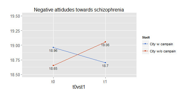
The idea to this function came up when we wanted to analyze the effect of an intervention (an educational programme on knowledge about mental disorders and associated stigma) between two groups: a “treatmeant” group (city) where a campaign on mental disorders was conducted and another city without this campaign. People from both cities were asked about their attitudes and knowledge about specific mental disorders at t0 before the campaign started in the one city. Some month later (t1), again people from both cities were asked the same questions. The intention was to see a) whether there were differences in knowledge and pro-social attidutes of people towards mental disorders and b) if the compaign successfully reduces stigma and increases knowledge.

To analyse these questions, we used an ANCOVA with knowledge and stigma score as dependent variables, “city” and “time” (t0 versus t1) as predictors and adjusted for covariates like age, sex, education etc. The estimated marginal means (or least-squares means) show you the differences of the dependent variable.

Here’s an example plot, quickly done with the sjp.emm.int function:

Since the data is not publicly available, I’ve set an an documentation with reproducable examples (though those example do not fit very well…).

The latest development snapshot of my package is available on GitHub.

BTW: You may have noticed that this function is quite similar to the sjp.lm.int function for visually interpreting interaction terms in linear models…

In the first part on visualizing (generalized) linear mixed effects models, I showed examples of the new functions in the sjPlot package to visualize fixed and random effects (estimates and odds ratios) of (g)lmer results. Meanwhile, I added further features to the functions, which I like to introduce here. This posting is based on the online manual of the sjPlot package.

In this posting, I’d like to give examples for diagnostic and probability plots of odds ratios. The latter examples, of course, only refer to the sjp.glmer function (generalized mixed models). To reproduce these examples, you need the version 1.59 (or higher) of the package, which can be found at GitHub. A submission to CRAN is planned for the next days…

Fitting example models

The following examples are based on two fitted mixed models:

# fit model
library(lme4)
# create binary response
sleepstudy$Reaction.dicho <- sju.dicho(sleepstudy$Reaction, 
                                       dichBy = "md")
# fit first model
fit <- glmer(Reaction.dicho ~ Days + (Days | Subject),
             sleepstudy,
             family = binomial("logit"))

data(efc)
# create binary response
efc$hi_qol <- sju.dicho(efc$quol_5)
# prepare group variable
efc$grp = as.factor(efc$e15relat)
levels(x = efc$grp) <- sji.getValueLabels(efc$e15relat)
# data frame for 2nd fitted model
mydf <- na.omit(data.frame(hi_qol = as.factor(efc$hi_qol),
                           sex = as.factor(efc$c161sex),
                           c12hour = as.numeric(efc$c12hour),
                           neg_c_7 = as.numeric(efc$neg_c_7),
                           grp = efc$grp))
# fit 2nd model
fit2 <- glmer(hi_qol ~ sex + c12hour + neg_c_7 + (1|grp),
              data = mydf,
              family = binomial("logit"))

Summary fit1

Formula: Reaction.dicho ~ Days + (Days | Subject)
   Data: sleepstudy

     AIC      BIC   logLik deviance df.resid 
   158.7    174.7    -74.4    148.7      175 

Scaled residuals: 
    Min      1Q  Median      3Q     Max 
-4.2406 -0.2726 -0.0198  0.2766  2.9705 

Random effects:
 Groups  Name        Variance Std.Dev. Corr 
 Subject (Intercept) 8.0287   2.8335        
         Days        0.2397   0.4896   -0.19
Number of obs: 180, groups:  Subject, 18

Fixed effects:
            Estimate Std. Error z value Pr(>|z|)    
(Intercept)  -3.8159     1.1728  -3.254 0.001139 ** 
Days          0.8908     0.2347   3.796 0.000147 ***
---
Signif. codes:  0 ‘***’ 0.001 ‘**’ 0.01 ‘*’ 0.05 ‘.’ 0.1 ‘ ’ 1

Correlation of Fixed Effects:
     (Intr)
Days -0.694

Summary fit2

Formula: hi_qol ~ sex + c12hour + neg_c_7 + (1 | grp)
   Data: mydf

     AIC      BIC   logLik deviance df.resid 
  1065.3   1089.2   -527.6   1055.3      881 

Scaled residuals: 
    Min      1Q  Median      3Q     Max 
-2.7460 -0.8139 -0.2688  0.7706  6.6464 

Random effects:
 Groups Name        Variance Std.Dev.
 grp    (Intercept) 0.08676  0.2945  
Number of obs: 886, groups:  grp, 8

Fixed effects:
             Estimate Std. Error z value Pr(>|z|)    
(Intercept)  3.179036   0.333940   9.520  < 2e-16 ***
sex2        -0.545282   0.178974  -3.047  0.00231 ** 
c12hour     -0.005148   0.001720  -2.992  0.00277 ** 
neg_c_7     -0.219586   0.024108  -9.109  < 2e-16 ***
---
Signif. codes:  0 ‘***’ 0.001 ‘**’ 0.01 ‘*’ 0.05 ‘.’ 0.1 ‘ ’ 1

Correlation of Fixed Effects:
        (Intr) sex2   c12hor
sex2    -0.410              
c12hour -0.057 -0.048       
neg_c_7 -0.765 -0.009 -0.116

Diagnostic plots

Two new functions are added to both sjp.lmer and sjp.glmer, hence they apply to linear and generalized linear mixed models, fitted with the lme4 package. The examples only refer to the sjp.glmer function.

Currently, there are two type options to plot diagnostic plots: type = "fe.cor" to plot a correlation matrix between fixed effects and type = "re.qq" to plot a qq-plot of random effects.

Correlation matrix of fixed effects

To plot a correlation matrix of the fixed effects, use type = "fe.cor".

# plot fixed effects correlation matrix
sjp.glmer(fit2, type = "fe.cor")

qq-plot of random effects

Another diagnostic plot is the qq-plot for random effects. Use type = "re.qq" to plot random against standard quantiles. The dots should be plotted along the line.

# plot qq-plot of random effects
sjp.glmer(fit, type = "re.qq")

Probability curves of odds ratios

These plotting functions have been implemented to easier interprete odds ratios, especially for continuous covariates, by plotting the probabilities of predictors.

Probabilities of fixed effects

With type = "fe.pc" (or type = "fe.prob"), probability plots for each covariate can be plotted. These probabilties are based on the fixed effects intercept. One plot per covariate is plotted.

The model fit2 has one binary and two continuous covariates:

# plot probability curve of fixed effects
sjp.glmer(fit2, type = "fe.pc")

Probabilities of fixed effects depending on grouping level (random intercept)

With type = "ri.pc" (or type = "ri.prob"), probability plots for each covariate can be plotted, depending on the grouping level from the random intercept. Thus, for each covariate a plot for each grouping levels is plotted. Furthermore, with the show.se the standard error of probabilities can be shown. In this example, only the plot for one covariate is shown, not for all.

# plot probability curves for each covariate
# grouped by random intercepts
sjp.glmer(fit2,
          type = "ri.pc",
          show.se = TRUE)

Instead of faceting plots, all grouping levels can be shown in one plot:

# plot probability curves for each covariate
# grouped by random intercepts
sjp.glmer(fit2,
          type = "ri.pc",
          facet.grid = FALSE)

Outlook

These will be the new features for the next package update. For later updates, I’m also planning to plot interaction terms of (generalized) linear mixed models, similar to the existing function for visualizing interaction terms in linear models.

My sjPlot package for data visualization has just been updated on CRAN. I’ve added some features to existing function, which I want to introduce here.

Plotting linear models

So far, plotting model assumptions of linear models or plotting slopes for each estimate of linear models were spread over several functions. Now, these plot types have been integrated into the sjp.lm function, where you can select the plot type with the type parameter. Furthermore, plotting standardized coefficients now also plot the related confidence intervals.

Detailed examples can be found here:
www.strengejacke.de/sjPlot/sjp.lm

Plotting generalized linear models

Beside odds ratios, you now can also plot the predicted probabilities of the outcome for each predictor of generalized linear models. In case you have continuous variables, these kind of plots may be more intuitive than an odds ratio value.

Detailed examples can be found here:
www.strengejacke.de/sjPlot/sjp.glm

Plotting (generalized) linear mixed effects models

The plotting function for creating plots of (generalized) linear mixed effects models (sjp.lmer and sjp.glmer) also got new plot types over the course of the last weeks.

For sjp.lmer, we have

• re (default) for estimates of random effects
• fe for estimates of fixed effects
• fe.std for standardized estimates of fixed effects
• fe.cor for correlation matrix of fixed effects
• re.qq for a QQ-plot of random effects (random effects quantiles against standard normal quantiles)
• fe.ri for fixed effects slopes depending on the random intercept.

and for sjp.glmer, we have

• re (default) for odds ratios of random effects
• fe for odds ratios of fixed effects
• fe.cor for correlation matrix of fixed effects
• re.qq for a QQ-plot of random effects (random effects quantiles against standard normal quantiles)
• fe.pc or fe.prob to plot probability curves (predicted probabilities) of all fixed effects coefficients. Use facet.grid to decide whether to plot each coefficient as separate plot or as integrated faceted plot.
• ri.pc or ri.prob to plot probability curves (predicted probabilities) of random intercept variances for all fixed effects coefficients. Use facet.grid to decide whether to plot each coefficient as separate plot or as integrated faceted plot.

Detailed examples can be found here:
www.strengejacke.de/sjPlot/sjp.lmer and www.strengejacke.de/sjPlot/sjp.glmer

Plotting interaction terms of (generalized) linear (mixed effects) models

Another function, where new features were added, is sjp.int (formerly known as sjp.lm.int). This function is now kind of generic and can plot interactions of

• linar models (lm)
• generalized linar models (glm)
• linar mixed effects models (lme4::lmer)
• generalized linar mixed effects models (lme4::glmer)

For linear models (both normal and mixed effects), slopes of interaction terms are plotted. For generalized linear models, the predicted probabilities of the outcome towards the interaction terms is plotted.

Detailed examples can be found here:
www.strengejacke.de/sjPlot/sjp.int

Plotting Likert scales

Finally, a comprehensive documentation for the sjp.likert function is finsihed, which can be found here:
www.strengejacke.de/sjPlot/sjp.likert

Hadley Wickham announced at Twitter that RStudio now provides CRAN package download logs. I was wondering about the download numbers of my package and wrote some code to extract that information from the logs…

The first code snippet is taken from the log website itself:

# Here's an easy way to get all the URLs in R
start <- as.Date('2013-11-28')
today <- as.Date('2015-03-04')

all_days <- seq(start, today, by = 'day')

year <- as.POSIXlt(all_days)$year + 1900
urls <- paste0('http://cran-logs.rstudio.com/', year, '/', all_days, '.csv.gz')

Then I downloaded all files into a folder:

for (i in 1:length(urls)) {
  download.file(urls[i], sprintf("~/Desktop/rstats/temp%i.csv.gz", i))
}

Unzipping did not work with unzip, so I just “opened” all files with the OS X unarchiver, which was quite convenient.

Than I read all csv-files and extracted the information for my package, sjPlot, from each csv-file and merged everything into one data frame:

sjPlot.df <- data.frame()
library(dplyr)
pb <- txtProgressBar(min=0, max=length(urls), style=3)

for (i in 1:length(urls)) {
  df.csv <- read.csv(sprintf("~/Desktop/rstats/temp%i.csv", i))
  pack <- tolower(as.character(df.csv$package))
  my.package <- which(pack == "sjplot")
  if (length(my.package) > 0 ) {
    dummy.df <- df.csv %>% dplyr::slice(my.package) %>% dplyr::select(date, package, version, country)
    sjPlot.df <- dplyr::bind_rows(sjPlot.df, dummy.df)
  }
  setTxtProgressBar(pb, i)
}
close(pb)
sjPlot.df$date.short <- strftime(sjPlot.df$date, format="%Y-%m")

Finally, the download-stats as plot:

library(sjPlot)
library(ggplot2)

mydf <- sjPlot.df %>% dplyr::count(date.short)

sjp.setTheme(theme = "539", axis.angle.x = 90)
ggplot(mydf, aes(x = date.short, y = n)) +
  geom_bar(stat = "identity", width = .5, alpha = .5, fill = "#3399cc") +
  scale_y_continuous(expand = c(0, 0), breaks = seq(250, 1500, 250)) +
  labs(x = sprintf("Monthly CRAN-downloads of sjPlot package since first release until 4th March (total download: %i)", sum(mydf$n)), y = NULL)

By the way, there’s already a shiny app for this…

My sjPlot package just reached version 2.0 and got many updates during the couple of last months. The focus was less on adding new functions; rather, I improved existing functions by adding new smaller and bigger features to make working with the package easier and more reliable. In this blog post, I will report some of the new features.

Consistent name style of arguments

Most notably, I tried to give all package functions a consistent naming style or pattern for arguments. In previous versions, mixing different name-styles was sometimes very confusing. For example, some functions used showNA, others na.rm or show.na. Or some functions used hideLegend, some showLegend and others again show.legend.

Now, all argument names are 1) lower case, 2) dot separated for longer words and are 3) grouped according to their function (i.e., if you open the docs for ?sjt.lm, you’ll find all show. arguments, then all string. and finally all digits. arguments). I know that this means that you most likely have to completely re-write your code that uses sjPlot-function calls, but I think, in the long run, this makes working with the sjPlot package easier

Support for different model families and link functions

In previous package versions, functions related to generalized linear models (like sjp.glm or sjp.glmer) were hard coded for binomial model families for most plot types. Some effect or prediction plots only worked for logistic regression, because predictions were based on plogis. Also, automatic entitling of plots always included „probability“, even for count models.

In the past package updates and especially and the last major update, prediction or effect plot are now based on the link-inverse function of the models, so all common model families and link functions should work with sjPlot now.

Predictions and effect plots

In some cases, it is easier to interprete the predicted probabilities, incidents rates or marginal effects instead of the related estimate numbers (odds ratios, incident rate ratios, beta). For linear models (sjp.lm), linear mixed models (sjp.lmer), generalized linear models (sjp.glm) and generalized linear mixed models (sjp.glmer), there are three different plot types to plot predicted values or marginal effects:

1. type = "slope" (or type = "fe.slope" and type = "ri.slope" for mixed models) to plot unadjusted predicted values, i.e. the relation between model terms and response.
2. type = "eff" to plot marginal effects, adjusted for all predictors.
3. type = "pred" (and type = "pred.fe" for mixed models) to plot predicted values against reponse, for particular model terms.

The following examples are taken from the vignette of the sjp.glm-function.

1. Predicted values, unadjusted

The predicted values from this plot type are based on the intercept’s estimate and each specific term’s estimate. All other co-variates are set to zero (i.e. ignored), which corresponds to family(fit)$linkinv(eta = b0 + bi * xi) (where xi is the estimate).

A probability curve of all predictors is plotted, which indicates the probability of the event (indicated by the response) occuring for each value of the predictor (not adjusted for remaining co-variates). In the above example, the first panel in the plot would be interpreted as: with increasing Barthel-Index (which means, better functional / physical status), the probability that caring for a dependent person is negatively perceived, decreases (in short: the less dependent a person I care for is, the less negative is the impact of care).

2. Effect plots

For marginal effects (predicted marginal probabilities resp. predicted marginal incident rates), all remaining co-variates are set to the mean, so this plot type adjusts for co-variates. Obtained results are based on the effects-package.

The effect plots can now also be non-faceted, and for selected model terms only (using the facit.grid and vars arguments).

3. Predicting values

The plot-type for predicting values did not produce any useful results in former package versions, because it just called the predict function without relationship to any predictor, or meaningful data. Now, this plot-type was completely revised. With type = "pred" (formerly, "y.pc"), you can plot predicted values for the response, related to specific model predictors. The predicted values of the response are computed, which corresponds to predict(fit, type = "response"). This plot type requires the vars argument to select specific terms that should be used for the x-axis and – optional – as grouping factor. Hence, vars must be a character vector with the names of one or two model predictors.

Table functions for mixed models

The table functions were also revised, especially for mixed models. You now have more details in the random parts section of the table, which now also shows the variance components of the random parts, or (pseudo-)r²-values.

The tables are created as HTML-page and displayed in your IDE’s viewer or your web browser. You can see many examples at the package vignettes-page. For the following example, I have taken a screenshot, because else the blog’s style sheet would break the table layout. Anyway, this is an example of a quickly produced table:

Closing remarks

There have been a lot of improvements made in the sjPlot package during the past update(s). Above you see example of the most obvious user-visible changes. But there were also lots of other smaller and bigger improvements. E.g. plotting functions with different plot types, like sjp.glm, have many arguments; most of them only applied to specific plot types, while they were ignored by other plot types. Now, all plot types support more or mostly all arguments, and the documentation should be clearer about what the functions and their arguments do.

I hope you’ll enjoy the sjPlot-package. Feel free to submit issues or suggestions to the dedicated GitHub-page.

Recent development in R packages are increasingly focussing on the philosophy of tidy data and a common package design and api. Tidy data is an important part of data exploration and analysis, as shown in the following figure:

Tidying data not only includes data cleaning, but also data transformation, both being necessary to perform the core steps of data analysis and visualization. This is a complex process, which involves many steps. You need many packages and functions to perfom those tasks. This is where a common package design and api comes into play: „A powerful strategy for solving complex problems is to combine many simple pieces“, says the tidyverse manifesto. For a coding workflow, this means:

• compose single functions with the pipe
• design your API so that it is easy to use by humans

The latter bullet point is helpful to achieve the first bullet point.

The sj-packages, namely sjPlot (data visualization), sjmisc (labelled data and data transformation) and sjstats (common statistical functions, also for regression modelling), are revised accordingly, to follow this design philosophy (as far as possible and feasible).

Pipe-friendly functions and tidy data

The „pipe-operator“ (%>%) was introduced by the magrittr-package and aims at a semantical change of your code, making reading and writing code more intuive. The %>% simply takes the left-hand side of an input and puts its result as first argument to the right-hand side.

library(sjmisc)
library(magrittr) # for pipe
data(efc)
# show head (first 6 observations) of efc-data
efc %>% head()

When doing data „tidying“ and transformation, the result of a left-hand side function is usually a data frame (for instance, when working with packages like dplyr or tidyr). Hence, the first argument of a function following the tidyverse-philosophy should always be the data.

In this blog post, I’ll focus on some functions of the sjPlot-package.

Using sjPlot in a pipe-workflow

The sjPlot-package for data visualization (see comprehensive documentation here) already included some functions that required the data as first argument (e.g. sjp.likert() or sjp.pca()). Other commonly used function, however, do not follow this design: sjp.frq() requires a vector, and sjp.xtab() requires two vectors, but no data frame, impossible to seamlessly integrate in a pipe-workflow.

library(sjmisc)
data(efc)
sjp.frq(efc$c172code)

The sjplot()-function

On the other hand, to quickly create figures for data exploration, it is often more feasible to just pass a vector to a function, instead of a prepared data frame. For this reason, I decided not to revise these functions and change their argument-structure. Instead, the latest sjPlot-update got a new wrapper function, sjplot(), which allows an easy integration of sjPlot-functions into a pipe-workflow. Since sjplot() is generic, you have to specify the plot-function via the fun-argument. The following code gives you the same figure as above:

library(sjmisc)
library(dplyr)
data(efc)
efc %>%
  select(c172code) %>%
  sjplot()

Functions that require multiple vectors as input – like sjp.scatter() or sjp.grpfrq() – work in the same manner:

efc %>%
  select(e17age, c172code, c161sex) %>%
  sjplot(fun = "scatter")

efc %>%
  select(e17age, c172code) %>%
  sjplot(fun = "grpfrq",
         type = "box",
         geom.colors = "Set1")

The plot_grid() function

Another convenient function is plot_grid(), which arranges multiple plots into a single grid-layout plot.

efc %>%
  select(e42dep, c172code, e16sex, c161sex) %>%
  sjplot() %>%
  plot_grid()

This function also accepts plot lists that are returned by some of the package’s function, which create multiple plots. It is an alternative to facetting plots. For example, plotting marginal effects of model predictors, by default arranges the plots in a facet-grid:

fit <- lm(tot_sc_e ~ c12hour + e17age +
          e42dep + neg_c_7, data = efc)
# plot marginal effects, as facet grid
sjp.lm(fit, type = "eff")

One disadvantage is the common axis-scale – all scales are continuous, although „dependency“ is a factor. Using plot_grid() solves this problem:

# plot marginal effects for each
# predictor, each as single plot
p <- sjp.lm(fit, type = "eff",
            facet.grid = FALSE,
            prnt.plot = FALSE)
# "p" has an element "$plot.list", which
# will automatically be used by plot_grid
plot_grid(p)

Final words

These were some examples of how to use the sjPlot-package in a pipe-workflow. Feel free to add your comments, further suggestions, either here or (preferably) at GitHub.

The next posting will cover new aspects of the sjmisc and sjstats packages.

My sjPlot-package was just updated on CRAN with some – as I think – useful new features.

First, I have added some vignettes to the package (based on the existing online-documentation) that cover some core features and principles of the sjPlot-package, so you have direct access to these manuals within R. The vignettes are also online on CRAN.

A second feature is the better support for black & white figures. There are two ways to create plots in black and white or greyscale. For bar plots, geom.colors = "gs" creates a plot using a greyscale (based on scales::grey_pal()).

library(sjPlot)
library(sjmisc)
library(ggplot2)
theme_set(theme_bw())
data(efc)
sjp.grpfrq(efc$e42dep, efc$c172code, geom.colors = "gs")

Similar to barplots, lineplots can be plotted in greyscale as well (with geom.colors = "gs"). However, in most cases lines colored in greyscale are difficult to distinguish. In this case, certain plot types in sjPlot support black & white figures with different linetypes.

Following plot-types allow black & white figures:

• sjp.grpfrq(type = „line“)
• sjp.int()
• sjp.lm(type = „pred“)
• sjp.glm(type = „pred“)
• sjp.lmer(type = „pred“)
• sjp.glmer(type = „pred“)

Use geom.colors = "bw" to create a b/w-plot.

# create binrary response
y <- ifelse(efc$neg_c_7 < median(na.omit(efc$neg_c_7)), 0, 1)
# create data frame for fitting model
df <- data.frame(
  y = to_factor(y),
  sex = to_factor(efc$c161sex),
  dep = to_factor(efc$e42dep),
  barthel = efc$barthtot,
  education = to_factor(efc$c172code)
)
# set variable label for response
set_label(df$y) <- "High Negative Impact"
# fit model
fit <- glm(y ~., data = df, family = binomial(link = "logit"))
# print predicted propbabilities
sjp.glm(fit, type = "pred", vars = c("barthel", "sex","dep"), geom.colors = "bw")

Different linetypes do not apply to other linetyped plots (like sjp.lm(type = "eff") or sjp.lm(type = "slope")), because these usually only plot a single line – so there’s no need for different linetypes, you can just set geom.colors = "black" (or geom.colors = "bw").

With this new feature, it’s pretty easy to create plots for (print) journals that require b/w or greyscaled figures.

I started writing my first package as collection of various functions that I needed for (almost) daily work. Meanwhile, packages were growing and bit by bit I sourced out functions to put them into new packages. Although this means more work for CRAN members when they have more packages to manage on their network, from a user-perspective it is much better if packages have a clear focus and a well defined set of functions. That’s why I now released a new package on CRAN, sjlabelled, which contains all functions that deal with labelled data. These functions use to live in the sjmisc-package, where they now are deprecated and will be removed in a future update.

My aim is not only to provide packages with a clear focus, but also with a consistent design and philosophy, making it easier and more intuitive to use (see also here) – I prefer to follow the so called „tidyverse“-approach here. It is still work in progress, but so far I think I’m on a good way…

So, what are the packages I use for (almost) daily work?

• sjlabelled – reading, writing and working with labelled data (especially since I collaborate a lot with people who use Stata or SPSS)
• sjmisc – data and variable transformation utilities (the complement to dplyr and tidyr, when it comes down from data frames to variables within the data wrangling process)
• sjstats – out-of-the-box statistics that is not already provided by base R or packages
• sjPlot – to quickly generate tables and plot
• ggeffects – to visualize regression models

The next step is creating cheat sheets for my packages. I think if you can map the scope and idea of your package (functions) on a cheat sheet, its focus is probably well defined.

Btw, if you also use some of the above packages more or less regularly, you can install the „strengejacke“-package to load them all in one step. This package is not on CRAN, because its only purpose is to load other packages.

Disclaimer: Of course I use other packages everyday as well – this posting is just focussing on my packages that I created because I frequently needed these kind of functions.

Some time ago I started working with Bayesian methods, using the great rstanarm-package. Beside the fantastic package-vignettes, and books like Statistical Rethinking or Doing Bayesion Data Analysis, I also found the ressources from Tristan Mahr helpful to both better understand Bayesian analysis and rstanarm. This motivated me to implement tools for Bayesian analysis into my packages, as well.

Due to the latest tidyr-update, I had to update some of my packages, in order to make them work again, so – beside some other features – some Bayes-stuff is now avaible in my packages on CRAN.

Finding shape or location parameters from distributions

The following functions are included in the sjstats-package. Given some known quantiles or percentiles, or a certain value or ratio and its standard error, the functions find_beta(), find_normal() or find_cauchy() help finding the parameters for a distribution. Taking the example from here, the plot indicates that the mean value for the normal distribution is somewhat above 50. We can find the exact parameters with find_normal(), using the information given in the text:

library(sjstats)
find_normal(x1 = 30, p1 = .1, x2 = 90, p2 = .8)
#> $mean
#> [1] 53.78387
#>
#> $sd
#> [1] 30.48026

High Density Intervals for MCMC samples

The hdi()-function computes the high density interval for posterior samples. This is nothing special, since there are other packages with such functions as well – however, you can use this function not only on vectors, but also on stanreg-objects (i.e. the results from models fitted with rstanarm). And, if required, you can also transform the HDI-values, e.g. if you need these intervals on an expontiated scale.

library(rstanarm)
fit <- stan_glm(mpg ~ wt + am, data = mtcars, chains = 1)
hdi(fit)
#>          term   hdi.low  hdi.high
#> 1 (Intercept) 32.158505 42.341421
#> 2          wt -6.611984 -4.022419
#> 3          am -2.567573  2.343818
#> 4       sigma  2.564218  3.903652

# fit logistic regression model
fit <- stan_glm(
  vs ~ wt + am,
  data = mtcars,
  family = binomial("logit"),
  chains = 1
)
hdi(fit, prob = .89, trans = exp)
#>          term      hdi.low     hdi.high
#> 1 (Intercept) 4.464230e+02 3.725603e+07
#> 2          wt 6.667981e-03 1.752195e-01
#> 3          am 8.923942e-03 3.747664e-01

Marginal effects for rstanarm-models

The ggeffects-package creates tidy data frames of model predictions, which are ready to use with ggplot (though there’s a plot()-method as well). ggeffects supports a wide range of models, and makes it easy to plot marginal effects for specific predictors, includinmg interaction terms. In the past updates, support for more model types was added, for instance polr (pkg MASS), hurdle and zeroinfl (pkg pscl), betareg (pkg betareg), truncreg (pkg truncreg), coxph (pkg survival) and stanreg (pkg rstanarm).

ggpredict() is the main function that computes marginal effects. Predictions for stanreg-models are based on the posterior distribution of the linear predictor (posterior_linpred()), mostly for convenience reasons. It is recommended to use the posterior predictive distribution (posterior_predict()) for inference and model checking, and you can do so using the ppd-argument when calling ggpredict(), however, especially for binomial or poisson models, it is harder (and much slower) to compute the „confidence intervals“. That’s why relying on posterior_linpred() is the default for stanreg-models with ggpredict().

Here is an example with two plots, one without raw data and one including data points:

library(sjmisc)
library(rstanarm)
library(ggeffects)
data(efc)
# make categorical
efc$c161sex <- to_label(efc$c161sex)

# fit model
m <- stan_glm(neg_c_7 ~ c160age + c12hour + c161sex, data = efc)
dat <- ggpredict(m, terms = c("c12hour", "c161sex"))
dat
#> # A tibble: 128 x 5
#>        x predicted conf.low conf.high  group
#>    <dbl>     <dbl>    <dbl>     <dbl> <fctr>
#>  1     4  10.80864 10.32654  11.35832   Male
#>  2     4  11.26104 10.89721  11.59076 Female
#>  3     5  10.82645 10.34756  11.37489   Male
#>  4     5  11.27963 10.91368  11.59938 Female
#>  5     6  10.84480 10.36762  11.39147   Male
#>  6     6  11.29786 10.93785  11.61687 Female
#>  7     7  10.86374 10.38768  11.40973   Male
#>  8     7  11.31656 10.96097  11.63308 Female
#>  9     8  10.88204 10.38739  11.40548   Male
#> 10     8  11.33522 10.98032  11.64661 Female
#> # ... with 118 more rows

plot(dat)
plot(dat, rawdata = TRUE)

As you can see, if you work with labelled data, the model-fitting functions from the rstanarm-package preserves all value and variable labels, making it easy to create annotated plots. The „confidence bands“ are actually hidh density intervals, computed with the above mentioned hdi()-function.

Next…

Next I will integrate ggeffects into my sjPlot-package, making sjPlot more generic and supporting more models types. Furthermore, sjPlot shall get a generic plot_model()-function which will replace former single functions like sjp.lm(), sjp.glm(), sjp.lmer() or sjp.glmer(). plot_model() should then produce a plot, either marginal effects, forest plots or interaction terms and so on, and accept (m)any model class. This should help making sjPlot more convenient to work with, more stable and easier to maintain…

Here’s a small preview of forthcoming features in the ggeffects-package, which are already available in the GitHub-version: For marginal effects from models fitted with glmmTMB() or glmer() resp. glmer.nb(), confidence intervals are now also computed.

If you want to test these features, simply install the package from GitHub:

library(devtools)
devtools::install_github("strengejacke/ggeffects")

Here are three examples:

library(glmmTMB)
library(lme4)
library(ggeffects)
data(Owls)

m1 <- glmmTMB(SiblingNegotiation ~ SexParent + ArrivalTime + (1 | Nest), data = Owls, family = nbinom1)
m2 <- glmmTMB(SiblingNegotiation ~ SexParent + ArrivalTime + (1 | Nest), data = Owls, family = nbinom2)
m3 <- glmer.nb(SiblingNegotiation ~ SexParent + ArrivalTime + (1 | Nest), data = Owls)
m4 <-
  glmmTMB(
    SiblingNegotiation ~ FoodTreatment + ArrivalTime + SexParent + (1 | Nest),
    data = Owls,
    ziformula =  ~ 1,
    family = list(family = "truncated_poisson", link = "log")
  )

pr1 <- ggpredict(m1, c("ArrivalTime", "SexParent"))
plot(pr1)

pr2 <- ggpredict(m2, c("ArrivalTime", "SexParent"))
plot(pr2)

pr3 <- ggpredict(m3, c("ArrivalTime", "SexParent"))
plot(pr3)

pr4 <- ggpredict(
  m4,
  c("FoodTreatment", "ArrivalTime [21,24,30]", "SexParent")
)
plot(pr4)

The code to calculate confidence intervals is based on the FAQ provided from Ben Bolker. Here is another example, that reproduces this plot (note, since age is numeric, ggpredict() produces a straight line, and not points with error bars).

library(nlme)
data(Orthodont)
m5 <- lmer(distance ~ age * Sex + (age|Subject), data = Orthodont)
pr5 <- ggpredict(m5, c("age", "Sex"))
plot(pr5)

I’m working on the next update of my sjPlot-package, which will get a generic plot_model() method, which plots any kind of regression model, with different plot types being supported (forest plots for estimates, marginal effects and predictions, including displaying interaction terms, …).

The package also supports rstan resp. rstanarm models. Since these are typically presented in a slightly different way (e.g., „outer“ and „inner“ probability of credible intervals), I implemented a special handling for these models, for which I wanted to show a quick preview here:

library(sjPlot)
library(rstanarm)

m <- stan_glm(
  mpg ~ cyl + disp + drat + wt + gear + am,
  data = mtcars
)

plot_model(m) + theme_sjplot()

The thin error bars represent the High Density Intervals (HDI) specified in the ci.lvl argument, the thick bar is the 50%-HDI, and the white point is the posterior median.

This is still work in progress, the latest version is on GitHub…